Special Functions
We will assume that our GP lets us plot multiple curves on the $xy$-plane by defining $y(x) = \; ... \;$ for each. We will also assume that it supports $\mathtt{pow, sqrt, log}$ as well as the basic the trigonometric functions $\mathtt{cos}$, $\mathtt{sin}$, $\mathtt{tan}$, $\mathtt{acos}$, $\mathtt{asin}$, $\mathtt{atan}$ out of the box. Some less standard functions include $\mathtt{abs, sgn, max, min}$. If our GP doesn't support these then we can define them in the following manner.
$$
\begin{array}{lll}
\mathtt{abs}(a) & = \sqrt(a^2) \\
\mathtt{sgn}(a) & = \frac{a}{|a|} \\
\mathtt{max}(a,b) &= \frac{1}{2} \left( a + b + |a-b| \right) \\
\mathtt{min}(a,b) &= \frac{1}{2} \left( a + b - |a-b| \right) \\
\end{array}
$$
Curve Segments
Suppose we want to plot only a segment of a curve, that is we want to restrict $\gamma$ to the domain $[a,b]$. If our GP lets us plot parametric equations then this is a simple matter. We define
$$
\begin{array}{llll}
x(t) = t \\
y(t) = \gamma(t) \\
t \in [a,b] \\
\end{array}
$$
Suppose however, that our GP only lets us plot $y$ as a function of $x$. How can we define $y(x) := \, ... $ so that it only plots $\gamma$ on the interval $x \in [a,b]$? Let's take a look at a concrete example. We have the two curves $\gamma: x \mapsto x+2$ and $\sigma: x \mapsto x(2x+1)$. Now we only want to plot the segment of $\gamma$ where $\gamma(x) \geq \sigma(x)$, ie. the interval $[-1,1]$. Here's how we can do it in GoodGrapher.

On the left we see the line $\gamma$ in blue in its full glory. On the right we see $\gamma$ restricted to the domain $[-1,1]$. The trick to plotting the segment is done by adding and subtracting $\mathtt{asin}(x)$. GoodGrapher fails to evaluate $\gamma$ outside $[-1,1]$ because $\mathtt{asin}(x)$ is undefined there. Generalizing, we let $\Omega_{I}$ be the set of all real-valued functions that have a (maximal) domain $I \subseteq \mathbb{R}^3$. This means that if $\omega \in \Omega_{I}$ then $\omega(x)$ is well-defined (real and bounded) $\mathtt{iff}$ $x \in I$. Combining functions by addition or composition yields the following rules.
$$
\begin{align}
\omega \quad & \in \quad \Omega_{I} \\
\phi \quad & \in \quad \Omega_{J} \\
\omega + \phi \quad & \in \quad \Omega_{\, I \, \cap \, J} \\
\omega \circ \phi \quad & \in \quad \Omega_{\, \{x \, \in\, J \; | \; \phi(x) \, \in \, I\}}
\end{align}
$$
Some examples include
$$
\begin{align}
\mathtt{asin}(x), \; \mathtt{acos}(x) \quad & \in \quad \Omega_{\, [-1,1]} \\
\; \sqrt{x+1}\, \sqrt{-x+1} \quad & \in \quad \Omega_{\, [-1,1]} \\
\sqrt{x} \quad & \in \quad \Omega_{\, [0,\infty)} \\
\mathtt{asin} \left( \tfrac{1}{b-a} (2x - a - b) \right) \quad & \in \quad \Omega_{\, [a,b]} \\
\mathtt{asin} \left( 2 \,\mathtt{cos}\, \pi x - 1 \right) \quad & \in \quad \Omega_{\, [0,1] \, \cup \, [2,3] \, \cup \, [4,5] \, \cup \, ...} \\
\mathtt{asin} (x^2 + y^2) \quad & \in \quad \Omega_{\,\mathbb{B}_2(1)}
\end{align}
$$
Notice how the composition-rule was used to define the function in $\Omega_{\, [a,b]}$. If we want to plot the segment $x \in [a,b]$ of the curve $\gamma$ we take any function $\omega \in \Omega_{[a,b]} $ and then simply define $y(x) := \gamma(x) + \omega(x) - \omega(x)$.
Curve Reflections
For example, reflecting about the line $y=0$ sends $(x,y) \mapsto (x,-y)$. Reflecting about the line $y=x$ sends $(x,y) \mapsto (y,x)$. Reflecting about $y = 1-x$ sends $(x,y) \mapsto (1-y,1-x)$. Plotting the reflected curve is straightforward in parametric form.

Curve Rotations

Combining Regions
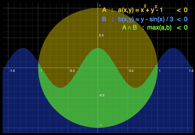
We will represent a region $F$ in the $xy$-plane canonically by $f(x,y) < 0$, where we may replace the $<$ with $\leq$ to include the boundary. For example, the inside of the circle centered at the origin with radius $1$ can be defined by $x^2 + y^2 - 1 < 0$. While GoodGrapher let's you shade such regions, it does not include a way to take the intersection or union. However, there is an easy workaround.
$$
\begin{align}
A \quad & : \quad a(x,y) < 0 \\
B \quad & : \quad b(x,y) < 0 \\
A \cap B \quad & : \quad \mathtt{max}(a,b) < 0 \\
A \cup B \quad & : \quad \mathtt{min}(a,b) < 0 \\
A \cup B - A \cap B \quad & : \quad ab < 0
\end{align}
$$

$$
\begin{array}{llll}
x(t) = t \\
y(t) = \gamma(t) \\
t \in [a,b] \\
\end{array}
$$
Suppose however, that our GP only lets us plot $y$ as a function of $x$. How can we define $y(x) := \, ... $ so that it only plots $\gamma$ on the interval $x \in [a,b]$? Let's take a look at a concrete example. We have the two curves $\gamma: x \mapsto x+2$ and $\sigma: x \mapsto x(2x+1)$. Now we only want to plot the segment of $\gamma$ where $\gamma(x) \geq \sigma(x)$, ie. the interval $[-1,1]$. Here's how we can do it in GoodGrapher.

On the left we see the line $\gamma$ in blue in its full glory. On the right we see $\gamma$ restricted to the domain $[-1,1]$. The trick to plotting the segment is done by adding and subtracting $\mathtt{asin}(x)$. GoodGrapher fails to evaluate $\gamma$ outside $[-1,1]$ because $\mathtt{asin}(x)$ is undefined there. Generalizing, we let $\Omega_{I}$ be the set of all real-valued functions that have a (maximal) domain $I \subseteq \mathbb{R}^3$. This means that if $\omega \in \Omega_{I}$ then $\omega(x)$ is well-defined (real and bounded) $\mathtt{iff}$ $x \in I$. Combining functions by addition or composition yields the following rules.
$$
\begin{align}
\omega \quad & \in \quad \Omega_{I} \\
\phi \quad & \in \quad \Omega_{J} \\
\omega + \phi \quad & \in \quad \Omega_{\, I \, \cap \, J} \\
\omega \circ \phi \quad & \in \quad \Omega_{\, \{x \, \in\, J \; | \; \phi(x) \, \in \, I\}}
\end{align}
$$
Some examples include
$$
\begin{align}
\mathtt{asin}(x), \; \mathtt{acos}(x) \quad & \in \quad \Omega_{\, [-1,1]} \\
\; \sqrt{x+1}\, \sqrt{-x+1} \quad & \in \quad \Omega_{\, [-1,1]} \\
\sqrt{x} \quad & \in \quad \Omega_{\, [0,\infty)} \\
\mathtt{asin} \left( \tfrac{1}{b-a} (2x - a - b) \right) \quad & \in \quad \Omega_{\, [a,b]} \\
\mathtt{asin} \left( 2 \,\mathtt{cos}\, \pi x - 1 \right) \quad & \in \quad \Omega_{\, [0,1] \, \cup \, [2,3] \, \cup \, [4,5] \, \cup \, ...} \\
\mathtt{asin} (x^2 + y^2) \quad & \in \quad \Omega_{\,\mathbb{B}_2(1)}
\end{align}
$$
Notice how the composition-rule was used to define the function in $\Omega_{\, [a,b]}$. If we want to plot the segment $x \in [a,b]$ of the curve $\gamma$ we take any function $\omega \in \Omega_{[a,b]} $ and then simply define $y(x) := \gamma(x) + \omega(x) - \omega(x)$.
Curve Reflections
Suppose we want to plot a curve reflected about a given line. Let our reflection line be $y = ax + b$. Upon reflection, the point $(x,y)$ gets mapped to
$$
\begin{align}
(x,y) \quad & \longmapsto \quad (\,\chi , \, \gamma\,) \\ \\
\chi(x,y) \quad & = \quad \tfrac{1}{a^2+1} \,[\,(1-a^2)x + 2ay -2ab\,] \\
\gamma(x,y) \quad & = \quad \tfrac{1}{a^2+1}\, [\,2ax + (a^2-1)y + 2b\,]
\end{align}
$$
$$
\begin{align}
(x,y) \quad & \longmapsto \quad (\,\chi , \, \gamma\,) \\ \\
\chi(x,y) \quad & = \quad \tfrac{1}{a^2+1} \,[\,(1-a^2)x + 2ay -2ab\,] \\
\gamma(x,y) \quad & = \quad \tfrac{1}{a^2+1}\, [\,2ax + (a^2-1)y + 2b\,]
\end{align}
$$

Curve Rotations
Suppose we want to rotate a curve about a given pivot $(p_x, p_y)$. Rotating the point $(x,y)$ counter-clockwise by an angle $\theta$ equates to the mapping.
$$
\begin{align}
x \quad & \mapsto \quad p_x \; + \; (x-p_x) \cos \theta \; - \; (y-p_y) \sin \theta \\
y \quad & \mapsto \quad p_y \; + \; (x-p_x) \sin \theta \; + \; (y-p_y) \cos \theta
\end{align}
$$
$$
\begin{align}
x \quad & \mapsto \quad p_x \; + \; (x-p_x) \cos \theta \; - \; (y-p_y) \sin \theta \\
y \quad & \mapsto \quad p_y \; + \; (x-p_x) \sin \theta \; + \; (y-p_y) \cos \theta
\end{align}
$$

Combining Regions
We will represent a region $F$ in the $xy$-plane canonically by $f(x,y) < 0$, where we may replace the $<$ with $\leq$ to include the boundary. For example, the inside of the circle centered at the origin with radius $1$ can be defined by $x^2 + y^2 - 1 < 0$. While GoodGrapher let's you shade such regions, it does not include a way to take the intersection or union. However, there is an easy workaround.
$$
\begin{align}
A \quad & : \quad a(x,y) < 0 \\
B \quad & : \quad b(x,y) < 0 \\
A \cap B \quad & : \quad \mathtt{max}(a,b) < 0 \\
A \cup B \quad & : \quad \mathtt{min}(a,b) < 0 \\
A \cup B - A \cap B \quad & : \quad ab < 0
\end{align}
$$
No comments:
Post a Comment